Specutils Documentation#
specutils is a Python package for representing, loading,
manipulating, and analyzing astronomical spectroscopic data. The
generic data containers and accompanying modules provide a toolbox that the
astronomical community can use to build more domain-specific packages. For more
details about the underlying principles, see
APE13, the
guiding document for spectroscopic development in the Astropy Project.
Changes in version 2#
The Spectrum1D class has been renamed to Spectrum to reduce confusion
about multi-dimensional flux arrays being supported. The current class name will be
deprecated in version 2.1; importing the old name will work but raise a deprecation
warning until then.
Single-dimensional flux use cases should be mostly unchanged in 2.0, with the exception being that spectrum arithmetic now checks that the spectral axis of both operands are equal, rather than simply checking that they are the same length. Thus, you will need to resample onto a common spectral axis if doing arithmetic on spectra with differing spectral axes.
Specutils version 2 implemented a major change in that Spectrum
no longer forces the spectral axis to be last for multi-dimensional data. This
was motivated by the desire for greater flexibility to allow for interoperability
with other packages that may wish to use specutils classes as the basis for
their own, and by the desire for consistency with the axis order that results
from a simple astropy.io.fits.read of a file. The legacy behavior can be
replicated by setting move_spectral_axis='last' when creating a new
Spectrum object. Spectrum will attempt to automatically
determine which flux axis corresponds to the spectral axis during initialization
based on the WCS (if provided) or the shape of the flux and spectral axis arrays,
but if the spectral axis index is unable to be automatically determined you will
need to specify which flux array axis is the dispersion axis with the
spectral_axis_index keyword. Note that since the spectral_axis can specify
either bin edges or bin centers, a flux array of shape (10,11) with spectral axis
of length 11 would be ambigious. In this case you could initialize a
Spectrum with bin_specification set to either “edges” or “centers”
to break the degeneracy.
An additional change for multi-dimensional spectra is that previously, initializing
such a Spectrum with a spectral_axis specified, but no WCS, would
create a Spectrum instance with a one-dimensional GWCS that was essentially
a lookup table with the spectral axis values. This case will now result in a GWCS with
dimensionality matching that of the flux array to facilitate use with downstream packages
that expect WCS dimensionality to match that of the data. The resulting spatial axes
transforms are simple pixel to pixel identity operations, since no actual spatial
coordinate information is available.
In addition to the changes to the generated GWCS, handling of input GWCS has also been
improved. This mostly manifests in the full GWCS (including spatial information) being
retained in the resulting Spectrum objects when reading, e.g., JWST spectral
cubes.
For a summary of the changes in version 2, you many also refer to the release notes.
Getting started with specutils#
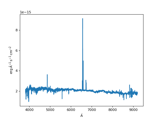
As a basic example, consider an emission line galaxy spectrum from the SDSS. We will use this as a proxy for a spectrum you may have downloaded from some archive, or reduced from your own observations.
We begin with some basic imports:
>>> from astropy.io import fits
>>> from astropy import units as u
>>> import numpy as np
>>> from matplotlib import pyplot as plt
>>> from astropy.visualization import quantity_support
>>> quantity_support()  # for getting units on the axes below
Now we load the dataset from its canonical source:
>>> filename = 'https://data.sdss.org/sas/dr16/sdss/spectro/redux/26/spectra/1323/spec-1323-52797-0012.fits'
>>> # The spectrum is in the second HDU of this file.
>>> with fits.open(filename) as f:
...     specdata = f[1].data
Then we re-format this dataset into astropy quantities, and create a
Spectrum object:
>>> from specutils import Spectrum
>>> lamb = 10**specdata['loglam'] * u.AA
>>> flux = specdata['flux'] * 10**-17 * u.Unit('erg cm-2 s-1 AA-1')
>>> spec = Spectrum(spectral_axis=lamb, flux=flux)
And we plot it:
>>> f, ax = plt.subplots()
>>> ax.step(spec.spectral_axis, spec.flux)
(Source code, png, hires.png, pdf)

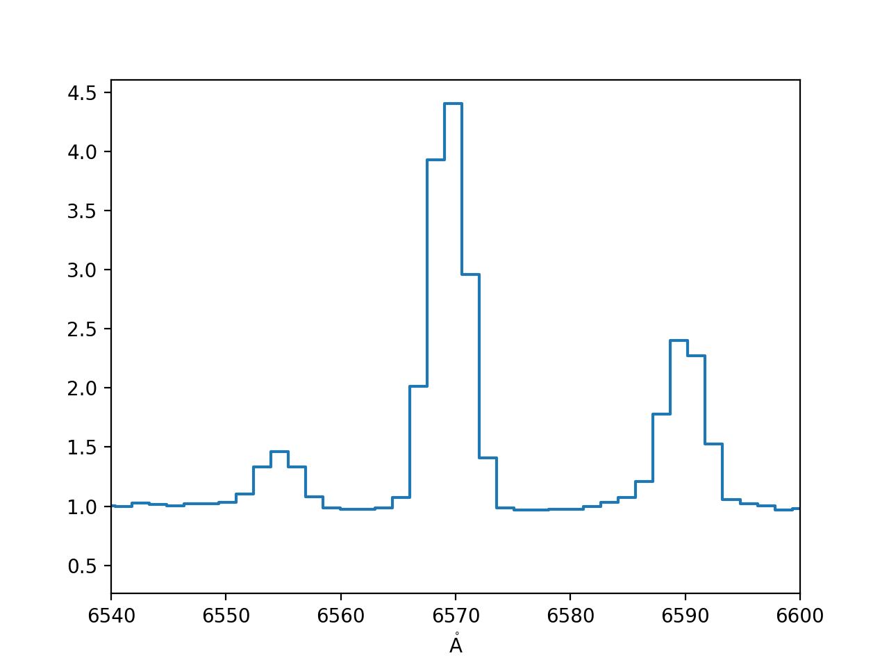
Now maybe you want the equivalent width of a spectral line. That requires normalizing by a continuum estimate:
>>> import warnings
>>> from specutils.fitting import fit_generic_continuum
>>> with warnings.catch_warnings():  # Ignore warnings
...     warnings.simplefilter('ignore')
...     cont_norm_spec = spec / fit_generic_continuum(spec)(spec.spectral_axis)
>>> f, ax = plt.subplots()
>>> ax.step(cont_norm_spec.wavelength, cont_norm_spec.flux)
>>> ax.set_xlim(654 * u.nm, 660 * u.nm)
But then you can apply a single function over the region of the spectrum containing the line:
>>> from specutils import SpectralRegion
>>> from specutils.analysis import equivalent_width
>>> equivalent_width(cont_norm_spec, regions=SpectralRegion(6562 * u.AA, 6575 * u.AA))
<Quantity -14.82013888 Angstrom>
(Source code, png, hires.png, pdf)

While there are other tools and spectral representations detailed more below, this gives a test of the sort of analysis specutils enables.
Using specutils#
For more details on usage of specutils, see the sections listed below.
- Installation
- Overview of How Specutils Represents Spectra
- Working with Spectrum objects
- Working With SpectrumCollections
- Working with Spectral Cubes
- Spectral Regions
- Analysis
- Line/Spectrum Fitting
- Manipulating Spectra
- Spectrum Arithmetic
- WCS Utilities
- Loading and Defining Custom Spectral File Formats
- Identifying Spectrum Formats
Get Involved - Developer Docs#
Please see Contributing for information on bug reporting and contributing to the specutils project.