Line/Spectrum Fitting#
One of the primary tasks in spectroscopic analysis is fitting models of spectra.
This concept is often applied mainly to line-fitting, but the same general
approach applies to continuum fitting or even full-spectrum fitting.
specutils provides conveniences that aim to leverage the general fitting
framework of astropy.modeling to spectral-specific tasks.
At a high level, this fitting takes the Spectrum object and a
list of Model objects that have initial guesses for each of
the parameters. these are used to create a compound model created from the model
initial guesses. This model is then actually fit to the spectrum’s flux,
yielding a single composite model result (which can be split back into its
components if desired).
Line Finding#
There are two techniques implemented in order to find emission and/or absorption
lines in a Spectrum spectrum.
The first technique is find_lines_threshold that will
find lines by thresholding the flux based on a factor applied to the
spectrum uncertainty. The second technique is
find_lines_derivative that will find the lines based
on calculating the derivative and then thresholding based on it. Both techniques
return an QTable that contains columns line_center,
line_type and line_center_index.
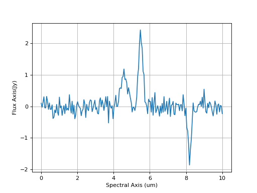
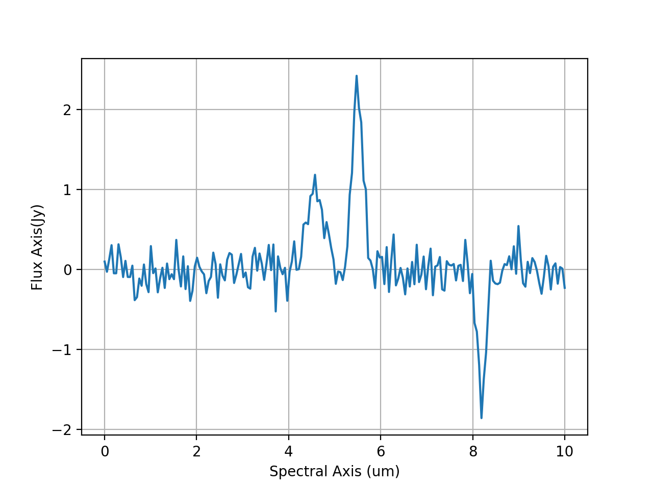
We start with a synthetic spectrum:
>>> import numpy as np
>>> from astropy.modeling import models
>>> import astropy.units as u
>>> from specutils import Spectrum, SpectralRegion
>>> np.random.seed(42)
>>> g1 = models.Gaussian1D(1, 4.6, 0.2)
>>> g2 = models.Gaussian1D(2.5, 5.5, 0.1)
>>> g3 = models.Gaussian1D(-1.7, 8.2, 0.1)
>>> x = np.linspace(0, 10, 200)
>>> y = g1(x) + g2(x) + g3(x) + np.random.normal(0., 0.2, x.shape)
>>> spectrum = Spectrum(flux=y*u.Jy, spectral_axis=x*u.um)
>>> from matplotlib import pyplot as plt
>>> plt.plot(spectrum.spectral_axis, spectrum.flux)
>>> plt.xlabel('Spectral Axis ({})'.format(spectrum.spectral_axis.unit))
>>> plt.ylabel('Flux Axis({})'.format(spectrum.flux.unit))
>>> plt.grid(True)
(Source code, png, hires.png, pdf)

While we know the true uncertainty here, this is often not the case with real
data. Therefore, since find_lines_threshold requires an
uncertainty, we will produce an estimate of the uncertainty by calling the
noise_region_uncertainty function:
>>> from specutils.manipulation import noise_region_uncertainty
>>> noise_region = SpectralRegion(0*u.um, 3*u.um)
>>> spectrum = noise_region_uncertainty(spectrum, noise_region)

>>> from specutils.fitting import find_lines_threshold
>>> lines = find_lines_threshold(spectrum, noise_factor=3)
>>> lines[lines['line_type'] == 'emission']
<QTable length=4>
   line_center    line_type line_center_index
        um
     float64        str10         int64
----------------- --------- -----------------
4.572864321608041  emission                91
4.824120603015076  emission                96
5.477386934673367  emission               109
 8.99497487437186  emission               179

>>> lines[lines['line_type'] == 'absorption']
<QTable length=1>
   line_center    line_type  line_center_index
        um
     float64        str10          int64
----------------- ---------- -----------------
8.190954773869347 absorption               163
An example using the find_lines_derivative:
>>> # Define a noise region for adding the uncertainty
>>> noise_region = SpectralRegion(0*u.um, 3*u.um)

>>> # Derivative technique
>>> from specutils.fitting import find_lines_derivative
>>> lines = find_lines_derivative(spectrum, flux_threshold=0.75)
>>> lines[lines['line_type'] == 'emission']
<QTable length=2>
   line_center    line_type line_center_index
        um
     float64        str10         int64
----------------- --------- -----------------
4.522613065326634  emission                90
5.477386934673367  emission               109

>>> lines[lines['line_type'] == 'absorption']
<QTable length=1>
   line_center    line_type  line_center_index
        um
     float64        str10          int64
----------------- ---------- -----------------
8.190954773869347 absorption               163
While it might be surprising that these tables do not contain more information
about the lines, this is because the “toolbox” philosophy of specutils aims to
keep such functionality in separate distinct functions. See Analysis for
functions that can be used to fill out common line measurements more
completely.
Parameter Estimation#
Given a spectrum with a set of lines, the estimate_line_parameters
can be called to estimate the Model parameters given a spectrum.
For the Gaussian1D,
Voigt1D, and
Lorentz1D models, there are predefined estimators for each
of the parameters. For all other models one must define the estimators (see example below).
Note that in many (most?) cases where another model is needed, it may be better to create
your own template models tailored to your specific spectra and skip this function entirely.
For example, based on the spectrum defined above we can first select a region:
>>> from specutils import SpectralRegion
>>> from specutils.fitting import estimate_line_parameters
>>> from specutils.manipulation import extract_region

>>> sub_region = SpectralRegion(4*u.um, 5*u.um)
>>> sub_spectrum = extract_region(spectrum, sub_region)
Then estimate the line parameters for a Gaussian line profile:
>>> result = estimate_line_parameters(sub_spectrum, models.Gaussian1D())
>>> print(result.amplitude)
Parameter('amplitude', value=1.1845669151078486, unit=Jy)

>>> print(result.mean)
Parameter('mean', value=4.57517271067525, unit=um)

>>> print(result.stddev)
Parameter('stddev', value=0.19373372929165977, unit=um, bounds=(1.1754943508222875e-38, None))
If an Model is used that does not have the predefined
parameter estimators, or if one wants to use different parameter estimators then
one can create a dictionary where the key is the parameter name and the value is
a function that operates on a spectrum (lambda functions are very useful for
this purpose). For example if one wants to estimate the line parameters of a
line fit for a RickerWavelet1D one can
define the estimators dictionary and use it to populate the estimator
attribute of the model’s parameters:
>>> from specutils import SpectralRegion
>>> from specutils.fitting import estimate_line_parameters
>>> from specutils.manipulation import extract_region
>>> from specutils.analysis import centroid, fwhm

>>> sub_region = SpectralRegion(4*u.um, 5*u.um)
>>> sub_spectrum = extract_region(spectrum, sub_region)

>>> ricker = models.RickerWavelet1D()
>>> ricker.amplitude.estimator = lambda s: max(s.flux)
>>> ricker.x_0.estimator = lambda *args: centroid(args[0], region=None)
>>> ricker.sigma.estimator = lambda *args: fwhm(args[0])

>>> estimate_line_parameters(spectrum, ricker)
<RickerWavelet1D(amplitude=2.4220684 Jy, x_0=3.60454769 um, sigma=0.24416769 um)>
Model (Line) Fitting#
The generic model fitting machinery is well-suited to fitting spectral lines. The first step is to create a set of models with initial guesses as the parameters. To achieve better fits it may be wise to include a set of bounds for each parameter, but that is optional.
Note
A method to make plausible initial guesses will be provided in a future version, but user defined initial guesses are required at present.
The fit_lines function takes as input the spectrum to be fit
and the set of models with initial guesses, and by default uses the
TRFLSQFitter to perform the fit. You may override
this by providing a different fitter to the fitter input parameter. Note
that the default fitter will populate the stds attribute of the returned
models with estimates of the standard deviation uncertainty in the fit parameters,
and that this may not be populated for user-defined non-default fitters. In general,
you can set calc_uncertainties=True when initializing an Astropy fitter to
return this information.
You can also retrieve the covariance matrices and other fit information from
which the uncertainties are calculated by setting get_fit_info=True in the
the call to fit_lines. This will populate fit_info
in the meta dictionary attached to the returned fitted model.
Below are a series of examples of this sort of fitting.
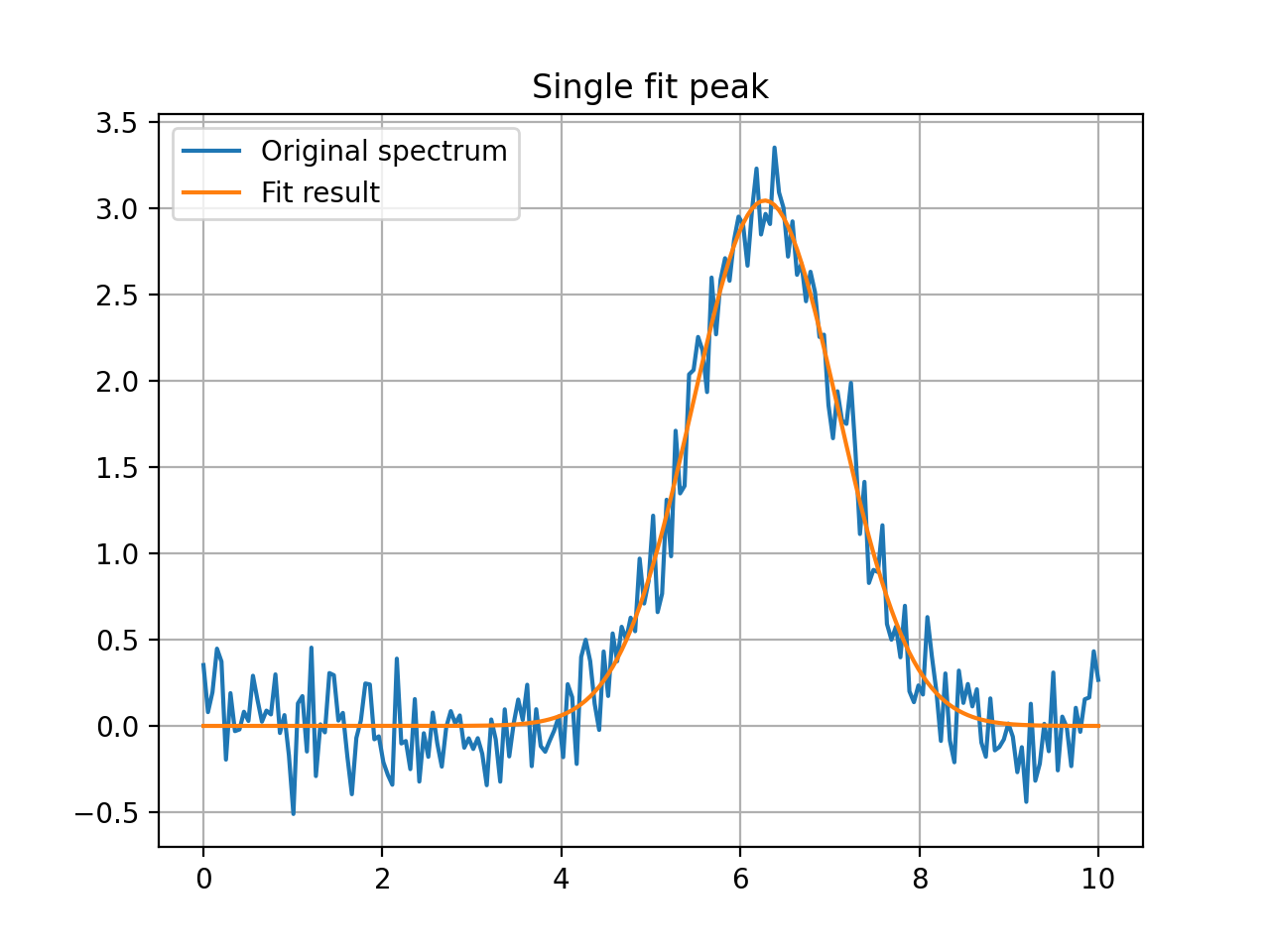
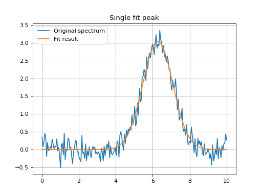
Simple Example#
Below is a simple example to demonstrate how to use the
fit_lines method to fit a spectrum to an Astropy model
initial guess.
import numpy as np
import matplotlib.pyplot as plt

from astropy.modeling import models
from astropy import units as u

from specutils.spectra import Spectrum
from specutils.fitting import fit_lines

# Create a simple spectrum with a Gaussian.
np.random.seed(0)
x = np.linspace(0., 10., 200)
y = 3 * np.exp(-0.5 * (x- 6.3)**2 / 0.8**2)
y += np.random.normal(0., 0.2, x.shape)
spectrum = Spectrum(flux=y*u.Jy, spectral_axis=x*u.um)

# Fit the spectrum and calculate the fitted flux values (``y_fit``)
g_init = models.Gaussian1D(amplitude=3.*u.Jy, mean=6.1*u.um, stddev=1.*u.um)
g_fit = fit_lines(spectrum, g_init)
y_fit = g_fit(x*u.um)

# Plot the original spectrum and the fitted.
plt.plot(x, y, label="Original spectrum")
plt.plot(x, y_fit, label="Fit result")
plt.title('Single fit peak')
plt.grid(True)
plt.legend()
(Source code, png, hires.png, pdf)
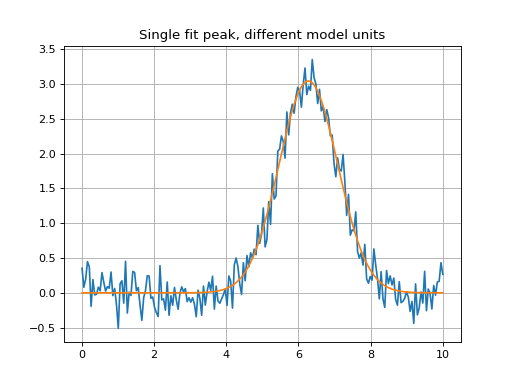
Simple Example with Different Units#
Similar fit example to above, but the Gaussian model initial guess has different units. The fit will convert the initial guess to the spectral units, fit and then output the fitted model in the spectrum units.
import numpy as np
import matplotlib.pyplot as plt

from astropy.modeling import models
from astropy import units as u

from specutils.spectra import Spectrum
from specutils.fitting import fit_lines

# Create a simple spectrum with a Gaussian.
np.random.seed(0)
x = np.linspace(0., 10., 200)
y = 3 * np.exp(-0.5 * (x- 6.3)**2 / 0.8**2)
y += np.random.normal(0., 0.2, x.shape)

# Create the spectrum
spectrum = Spectrum(flux=y*u.Jy, spectral_axis=x*u.um)

# Fit the spectrum
g_init = models.Gaussian1D(amplitude=3.*u.Jy, mean=61000*u.AA, stddev=10000.*u.AA)
g_fit = fit_lines(spectrum, g_init)
y_fit = g_fit(x*u.um)

plt.plot(x, y)
plt.plot(x, y_fit)
plt.title('Single fit peak, different model units')
plt.grid(True)
(Source code, png, hires.png, pdf)

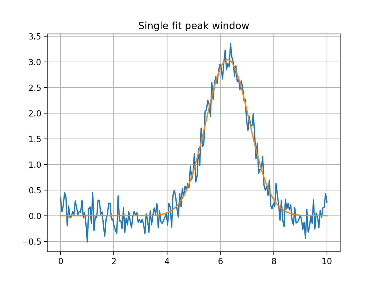
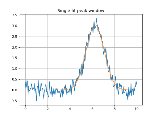
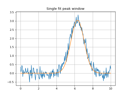
Single Peak Fit Within a Window (Defined by Center)#
Single peak fit with a window of 2*u.um around the center of the
mean of the model initial guess (so 2*u.um around 5.5*u.um).
import numpy as np
import matplotlib.pyplot as plt

from astropy.modeling import models
from astropy import units as u

from specutils.spectra import Spectrum
from specutils.fitting import fit_lines

# Create a simple spectrum with a Gaussian.
np.random.seed(0)
x = np.linspace(0., 10., 200)
y = 3 * np.exp(-0.5 * (x- 6.3)**2 / 0.8**2)
y += np.random.normal(0., 0.2, x.shape)

# Create the spectrum
spectrum = Spectrum(flux=y*u.Jy, spectral_axis=x*u.um)

# Fit the spectrum
g_init = models.Gaussian1D(amplitude=3.*u.Jy, mean=5.5*u.um, stddev=1.*u.um)
g_fit = fit_lines(spectrum, g_init, window=2*u.um)
y_fit = g_fit(x*u.um)

plt.plot(x, y)
plt.plot(x, y_fit)
plt.title('Single fit peak window')
plt.grid(True)
(Source code, png, hires.png, pdf)
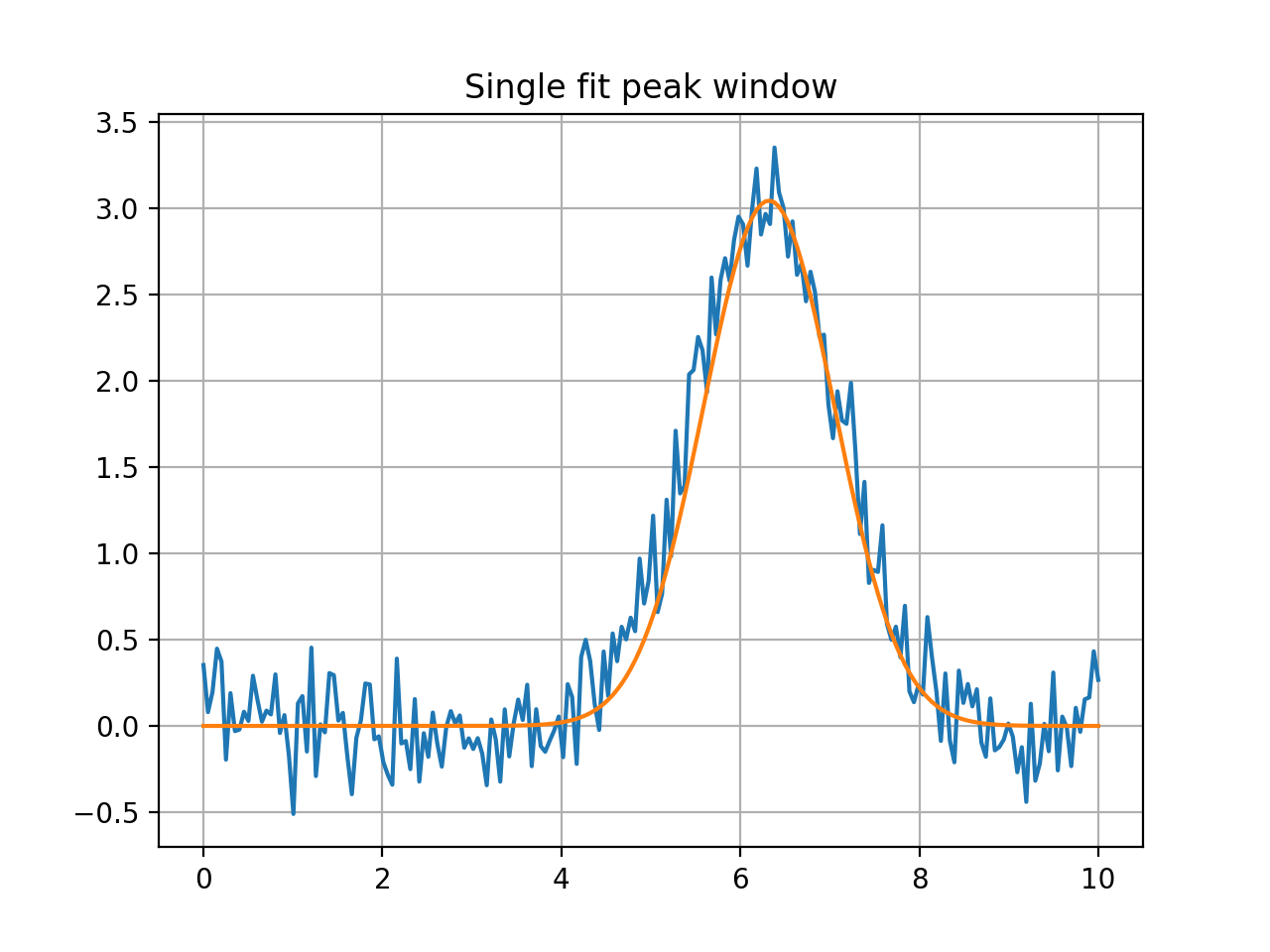
Single Peak Fit Within a Window (Defined by Left and Right)#
Single peak fit using spectral data only within the window
6*u.um to 7*u.um, all other data will be ignored.
import numpy as np
import matplotlib.pyplot as plt

from astropy.modeling import models
from astropy import units as u

from specutils.spectra import Spectrum
from specutils.fitting import fit_lines

# Create a simple spectrum with a Gaussian.
np.random.seed(0)
x = np.linspace(0., 10., 200)
y = 3 * np.exp(-0.5 * (x- 6.3)**2 / 0.8**2)
y += np.random.normal(0., 0.2, x.shape)

# Create the spectrum
spectrum = Spectrum(flux=y*u.Jy, spectral_axis=x*u.um)

# Fit the spectrum
g_init = models.Gaussian1D(amplitude=3.*u.Jy, mean=5.5*u.um, stddev=1.*u.um)
g_fit = fit_lines(spectrum, g_init, window=(6*u.um, 7*u.um))
y_fit = g_fit(x*u.um)

plt.plot(x, y)
plt.plot(x, y_fit)
plt.title('Single fit peak window')
plt.grid(True)
(Source code, png, hires.png, pdf)
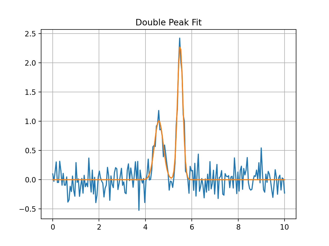
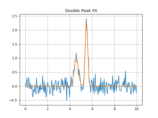
Double Peak Fit#
Double peak fit compound model initial guess in and compound model out.
import numpy as np
import matplotlib.pyplot as plt

from astropy.modeling import models
from astropy import units as u

from specutils.spectra import Spectrum
from specutils.fitting import fit_lines

# Create a simple spectrum with a Gaussian.
np.random.seed(42)

g1 = models.Gaussian1D(1, 4.6, 0.2)
g2 = models.Gaussian1D(2.5, 5.5, 0.1)
x = np.linspace(0, 10, 200)
y = g1(x) + g2(x) + np.random.normal(0., 0.2, x.shape)

# Create the spectrum to fit
spectrum = Spectrum(flux=y*u.Jy, spectral_axis=x*u.um)

# Fit the spectrum
g1_init = models.Gaussian1D(amplitude=2.3*u.Jy, mean=5.6*u.um, stddev=0.1*u.um)
g2_init = models.Gaussian1D(amplitude=1.*u.Jy, mean=4.4*u.um, stddev=0.1*u.um)
g12_fit = fit_lines(spectrum, g1_init+g2_init)
y_fit = g12_fit(x*u.um)

plt.plot(x, y)
plt.plot(x, y_fit)
plt.title('Double Peak Fit')
plt.grid(True)
(Source code, png, hires.png, pdf)
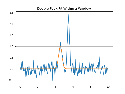
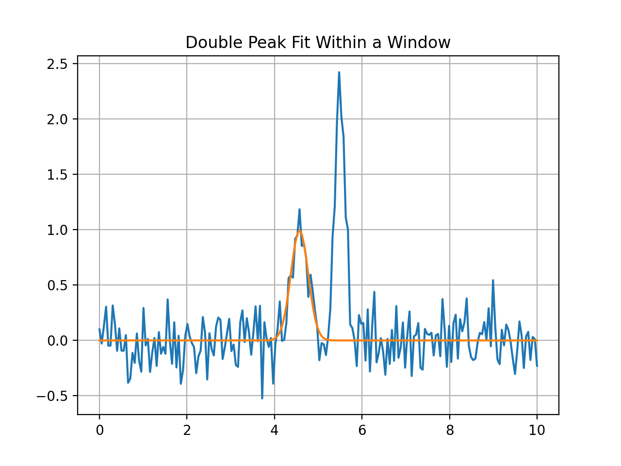
Double Peak Fit Within a Window#
Double peak fit using data in the spectrum from 4.3*u.um to 5.3*u.um, only.
import numpy as np
import matplotlib.pyplot as plt

from astropy.modeling import models
from astropy import units as u

from specutils.spectra import Spectrum
from specutils.fitting import fit_lines

# Create a simple spectrum with a Gaussian.
np.random.seed(42)

g1 = models.Gaussian1D(1, 4.6, 0.2)
g2 = models.Gaussian1D(2.5, 5.5, 0.1)
x = np.linspace(0, 10, 200)
y = g1(x) + g2(x) + np.random.normal(0., 0.2, x.shape)

# Create the spectrum to fit
spectrum = Spectrum(flux=y*u.Jy, spectral_axis=x*u.um)

# Fit the spectrum
g2_init = models.Gaussian1D(amplitude=1.*u.Jy, mean=4.7*u.um, stddev=0.2*u.um)
g2_fit = fit_lines(spectrum, g2_init, window=(4.3*u.um, 5.3*u.um))
y_fit = g2_fit(x*u.um)

plt.plot(x, y)
plt.plot(x, y_fit)
plt.title('Double Peak Fit Within a Window')
plt.grid(True)
(Source code, png, hires.png, pdf)

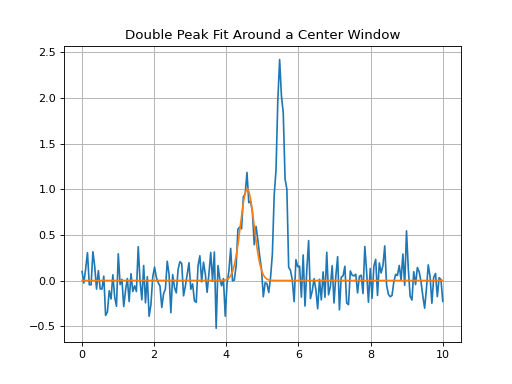
Double Peak Fit Within Around a Center Window#
Double peak fit using data in the spectrum centered on 4.7*u.um +/- 0.3*u.um.
import numpy as np
import matplotlib.pyplot as plt

from astropy.modeling import models
from astropy import units as u

from specutils.spectra import Spectrum
from specutils.fitting import fit_lines

# Create a simple spectrum with a Gaussian.
np.random.seed(42)

g1 = models.Gaussian1D(1, 4.6, 0.2)
g2 = models.Gaussian1D(2.5, 5.5, 0.1)
x = np.linspace(0, 10, 200)
y = g1(x) + g2(x) + np.random.normal(0., 0.2, x.shape)

# Create the spectrum to fit
spectrum = Spectrum(flux=y*u.Jy, spectral_axis=x*u.um)

# Fit the spectrum
g2_init = models.Gaussian1D(amplitude=1.*u.Jy, mean=4.7*u.um, stddev=0.2*u.um)
g2_fit = fit_lines(spectrum, g2_init, window=0.3*u.um)
y_fit = g2_fit(x*u.um)

plt.plot(x, y)
plt.plot(x, y_fit)
plt.title('Double Peak Fit Around a Center Window')
plt.grid(True)
(Source code, png, hires.png, pdf)

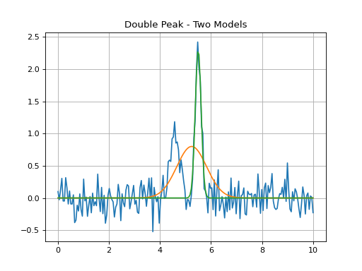
Double Peak Fit - Two Separate Peaks#
Double peak fit where each model gl_init and gr_init is fit separately,
each within 0.2*u.um of the model’s mean.
import numpy as np
import matplotlib.pyplot as plt

from astropy.modeling import models
from astropy import units as u

from specutils.spectra import Spectrum
from specutils.fitting import fit_lines

# Create a simple spectrum with a Gaussian.
np.random.seed(42)

g1 = models.Gaussian1D(1, 4.6, 0.2)
g2 = models.Gaussian1D(2.5, 5.5, 0.1)
x = np.linspace(0, 10, 200)
y = g1(x) + g2(x) + np.random.normal(0., 0.2, x.shape)

# Create the spectrum to fit
spectrum = Spectrum(flux=y*u.Jy, spectral_axis=x*u.um)

# Fit each peak
gl_init = models.Gaussian1D(amplitude=1.*u.Jy, mean=4.8*u.um, stddev=0.2*u.um)
gr_init = models.Gaussian1D(amplitude=2.*u.Jy, mean=5.3*u.um, stddev=0.2*u.um)
gl_fit, gr_fit = fit_lines(spectrum, [gl_init, gr_init], window=0.2*u.um)
yl_fit = gl_fit(x*u.um)
yr_fit = gr_fit(x*u.um)

plt.plot(x, y)
plt.plot(x, yl_fit)
plt.plot(x, yr_fit)
plt.title('Double Peak - Two Models')
plt.grid(True)
(Source code, png, hires.png, pdf)
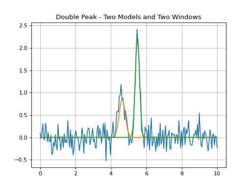
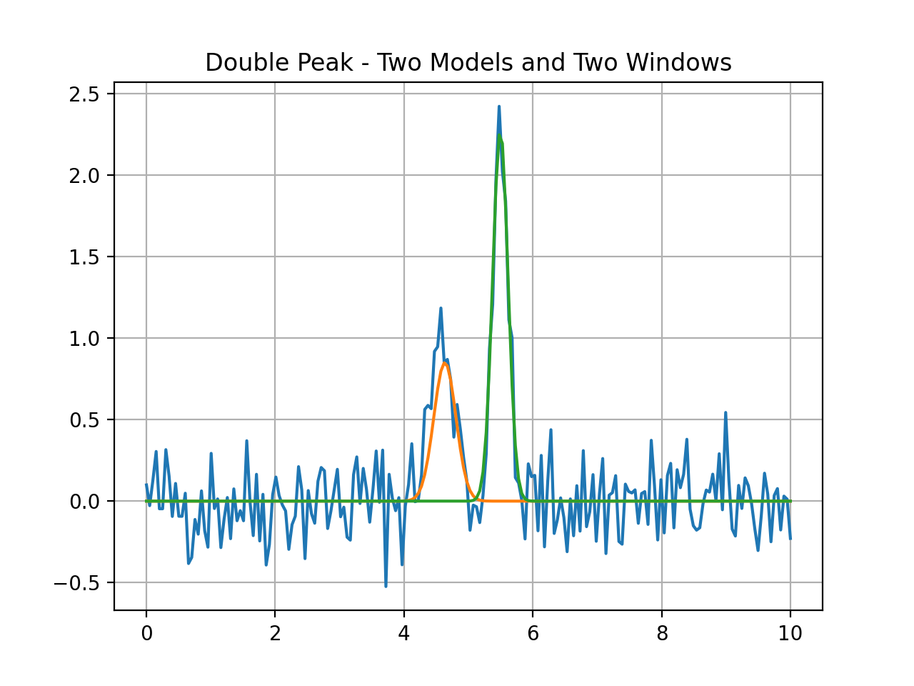
Double Peak Fit - Two Separate Peaks With Two Windows#
Double peak fit where each model gl_init and gr_init is fit within
the corresponding window.
>>> import numpy as np
>>> import matplotlib.pyplot as plt
>>> from astropy.modeling import models
>>> from astropy import units as u
>>> from specutils.spectra import Spectrum
>>> from specutils.fitting import fit_lines
>>> # Create a simple spectrum with a Gaussian.
>>> np.random.seed(42)
>>> g1 = models.Gaussian1D(1, 4.6, 0.2)
>>> g2 = models.Gaussian1D(2.5, 5.5, 0.1)
>>> x = np.linspace(0, 10, 200)
>>> y = g1(x) + g2(x) + np.random.normal(0., 0.2, x.shape)
>>> # Create the spectrum to fit
>>> spectrum = Spectrum(flux=y*u.Jy, spectral_axis=x*u.um)
>>> # Fit each peak
>>> gl_init = models.Gaussian1D(amplitude=1.*u.Jy, mean=4.8*u.um, stddev=0.2*u.um)
>>> gr_init = models.Gaussian1D(amplitude=2.*u.Jy, mean=5.3*u.um, stddev=0.2*u.um)
>>> gl_fit, gr_fit = fit_lines(spectrum, [gl_init, gr_init], window=[(4.6*u.um, 5.3*u.um), (5.3*u.um, 5.8*u.um)])
>>> yl_fit = gl_fit(x*u.um)
>>> yr_fit = gr_fit(x*u.um)
>>> f, ax = plt.subplots()
>>> ax.plot(x, y)
>>> ax.plot(x, yl_fit)
>>> ax.plot(x, yr_fit)
>>> ax.set_title("Double Peak - Two Models and Two Windows")
>>> ax.grid(True)
(Source code, png, hires.png, pdf)

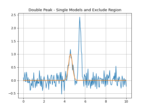
Double Peak Fit - Exclude One Region#
Double peak fit where each model gl_init and gr_init is fit using
all the data except between 5.2*u.um and 5.8*u.um.
>>> import numpy as np
>>> import matplotlib.pyplot as plt
>>> from astropy.modeling import models
>>> from astropy import units as u
>>> from specutils.spectra import Spectrum, SpectralRegion
>>> from specutils.fitting import fit_lines
>>> # Create a simple spectrum with a Gaussian.
>>> np.random.seed(42)
>>> g1 = models.Gaussian1D(1, 4.6, 0.2)
>>> g2 = models.Gaussian1D(2.5, 5.5, 0.1)
>>> x = np.linspace(0, 10, 200)
>>> y = g1(x) + g2(x) + np.random.normal(0., 0.2, x.shape)
>>> # Create the spectrum to fit
>>> spectrum = Spectrum(flux=y*u.Jy, spectral_axis=x*u.um)
>>> # Fit each peak
>>> gl_init = models.Gaussian1D(amplitude=1.*u.Jy, mean=4.8*u.um, stddev=0.2*u.um)
>>> gl_fit = fit_lines(spectrum, gl_init, exclude_regions=[SpectralRegion(5.2*u.um, 5.8*u.um)])
>>> yl_fit = gl_fit(x*u.um)
>>> f, ax = plt.subplots()
>>> ax.plot(x, y)
>>> ax.plot(x, yl_fit)
>>> ax.set_title("Double Peak - Single Models and Exclude Region")
>>> ax.grid(True)
(Source code, png, hires.png, pdf)
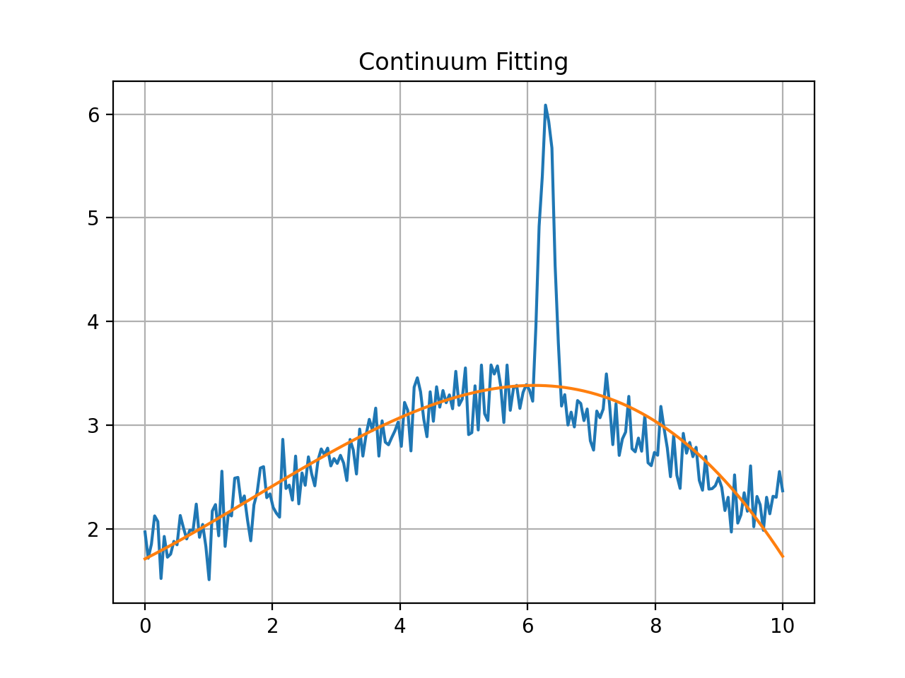
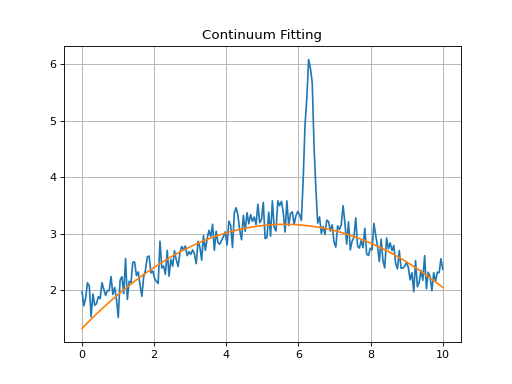
Continuum Fitting#
While the line-fitting machinery can be used to fit continuua at the same time
as models, often it is convenient to subtract or normalize a spectrum by its
continuum before other processing is done. specutils provides some
convenience functions to perform exactly this task. An example is shown below.
>>> import warnings
>>> import numpy as np
>>> import matplotlib.pyplot as plt
>>> from astropy.modeling import models
>>> from astropy import units as u
>>> from specutils.spectra import Spectrum, SpectralRegion
>>> from specutils.fitting import fit_generic_continuum
>>> np.random.seed(0)
>>> x = np.linspace(0., 10., 200)
>>> y = 3 * np.exp(-0.5 * (x - 6.3)**2 / 0.1**2)
>>> y += np.random.normal(0., 0.2, x.shape)
>>> y_continuum = 3.2 * np.exp(-0.5 * (x - 5.6)**2 / 4.8**2)
>>> y += y_continuum
>>> spectrum = Spectrum(flux=y*u.Jy, spectral_axis=x*u.um)
>>> with warnings.catch_warnings():  # Ignore warnings
...     warnings.simplefilter('ignore')
...     g1_fit = fit_generic_continuum(spectrum)
>>> y_continuum_fitted = g1_fit(x*u.um)
>>> f, ax = plt.subplots()
>>> ax.plot(x, y)
>>> ax.plot(x, y_continuum_fitted)
>>> ax.set_title("Continuum Fitting")
>>> ax.grid(True)
(Source code, png, hires.png, pdf)
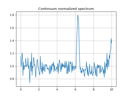
The normalized spectrum is simply the old spectrum devided by the fitted continuum, which returns a new object:
>>> spec_normalized = spectrum / y_continuum_fitted
>>> f, ax = plt.subplots()
>>> ax.plot(spec_normalized.spectral_axis, spec_normalized.flux)
>>> ax.set_title("Continuum normalized spectrum")
>>> ax.grid(True)
(Source code, png, hires.png, pdf)
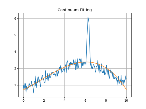
When fitting over a specific wavelength region of a spectrum, one
should use the window parameter to specify the region. Windows
can be comprised of more than one wavelength interval; each interval
is specified by a sequence:
>>> import warnings
>>> import numpy as np
>>> import matplotlib.pyplot as plt
>>> import astropy.units as u
>>> from specutils.spectra.spectrum import Spectrum
>>> from specutils.fitting.continuum import fit_continuum
>>> np.random.seed(0)
>>> x = np.linspace(0., 10., 200)
>>> y = 3 * np.exp(-0.5 * (x - 6.3) ** 2 / 0.1 ** 2)
>>> y += np.random.normal(0., 0.2, x.shape)
>>> y += 3.2 * np.exp(-0.5 * (x - 5.6) ** 2 / 4.8 ** 2)
>>> spectrum = Spectrum(flux=y * u.Jy, spectral_axis=x * u.um)
>>> region = [(1 * u.um, 5 * u.um), (7 * u.um, 10 * u.um)]
>>> with warnings.catch_warnings():  # Ignore warnings
...     warnings.simplefilter('ignore')
...     fitted_continuum = fit_continuum(spectrum, window=region)
>>> y_fit = fitted_continuum(x*u.um)
>>> f, ax = plt.subplots()
>>> ax.plot(x, y)
>>> ax.plot(x, y_fit)
>>> ax.set_title("Continuum Fitting")
>>> plt.grid(True)
(Source code, png, hires.png, pdf)

Reference/API#
Functions#
|
The input |
|
Find the emission and absorption lines in a spectrum. |
|
Find the emission and absorption lines in a spectrum. |
|
Entry point for fitting using the |
|
Basic fitting of the continuum of an input spectrum. |
|
Fit the input models to the spectrum. |