Analysis¶

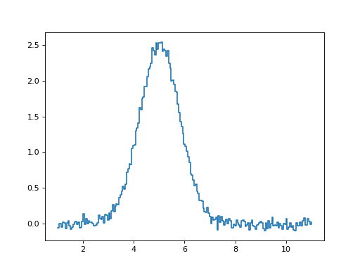
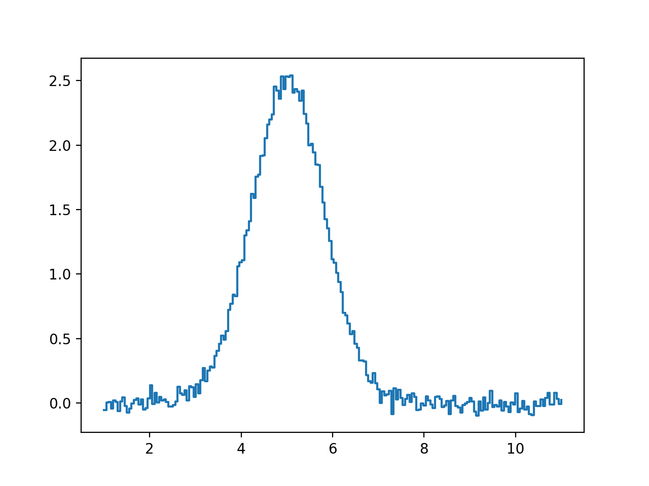
The specutils package comes with a set of tools for doing common analysis tasks on astronomical spectra. Some examples of applying these tools are described below. The basic spectrum shown here is used in the examples in the sub-sections below - a gaussian-profile line with flux of 5 GHz Jy. See Working with Spectrum1Ds for more on creating spectra:

>>> import numpy as np
>>> from astropy import units as u
>>> from astropy.nddata import StdDevUncertainty
>>> from astropy.modeling import models
>>> from specutils import Spectrum1D, SpectralRegion
>>> np.random.seed(42)
>>> spectral_axis = np.linspace(11., 1., 200) * u.GHz
>>> spectral_model = models.Gaussian1D(amplitude=5*(2*np.pi*0.8**2)**-0.5*u.Jy, mean=5*u.GHz, stddev=0.8*u.GHz)
>>> flux = spectral_model(spectral_axis)
>>> flux += np.random.normal(0., 0.05, spectral_axis.shape) * u.Jy
>>> uncertainty = StdDevUncertainty(0.2*np.ones(flux.shape)*u.Jy)
>>> noisy_gaussian = Spectrum1D(spectral_axis=spectral_axis, flux=flux, uncertainty=uncertainty)
>>> import matplotlib.pyplot as plt 
>>> plt.step(noisy_gaussian.spectral_axis, noisy_gaussian.flux) 

(Source code, png, hires.png, pdf)

SNR¶

The signal-to-noise ratio of a spectrum is often a valuable quantity for evaluating the quality of a spectrum. The snr function performs this task, either on the spectrum as a whole, or sub-regions of a spectrum:

>>> from specutils.analysis import snr
>>> snr(noisy_gaussian)  
<Quantity 2.47730726>
>>> snr(noisy_gaussian, SpectralRegion(6*u.GHz, 4*u.GHz))  
<Quantity 9.8300873>

A second method to calculate SNR does not require the uncertainty defined on the Spectrum1D object. This computes the signal to noise ratio DER_SNR following the definition set forth by the Spectral Container Working Group of ST-ECF, MAST and CADC. This algorithm is described at https://esahubble.org/static/archives/stecfnewsletters/pdf/hst_stecf_0042.pdf

>>> from specutils.analysis import snr_derived
>>> snr_derived(noisy_gaussian)  
<Quantity 1.13359867>
>>> snr_derived(noisy_gaussian, SpectralRegion(6*u.GHz, 4*u.GHz))  
<Quantity 42.10020601>

The conditions on the data for this implementation for it to be an unbiased estimator of the SNR are strict. In particular:

the noise is uncorrelated in wavelength bins spaced two pixels apart

for large wavelength regions, the signal over the scale of 5 or more pixels can be approximated by a straight line

Line Flux Estimates¶

While line-fitting (see Line/Spectrum Fitting) is a more thorough way to measure spectral line fluxes, direct measures of line flux are very useful for either quick-look settings or for spectra not amedable to fitting. The line_flux function addresses that use case. The closely related specutils.analysis.equivalent_width computes the equivalent width of a spectral feature, a flux measure that is normalized against the continuum of a spectrum. Both are demonstrated below:

Note

The line_flux function assumes the spectrum has already been continuum-subtracted, while equivalent_width assumes the continuum is at a fixed, known level (defaulting to 1, meaning continuum-normalized). Continuum Fitting describes how continuua can be generated to prepare a spectrum for use with these functions.

>>> from specutils.analysis import line_flux
>>> line_flux(noisy_gaussian, SpectralRegion(7*u.GHz, 3*u.GHz))  
<Quantity 4.93784874 GHz Jy>
>>> line_flux(noisy_gaussian).to(u.erg * u.cm**-2 * u.s**-1)  
<Quantity 4.97951087e-14 erg / (s cm2)>

These line_flux measurements also include uncertainties if the spectrum itself has uncertainties:

>>> flux = line_flux(noisy_gaussian)
>>> flux.uncertainty.to(u.erg * u.cm**-2 * u.s**-1) 
<Quantity 1.42132016e-15 erg / (s cm2)>
>>> line_flux(noisy_gaussian, SpectralRegion(7*u.GHz, 3*u.GHz))  
<Quantity 4.93784874 GHz Jy>

For the equivalent width, note the need to add a continuum level:

>>> from specutils.analysis import equivalent_width
>>> noisy_gaussian_with_continuum = noisy_gaussian + 1*u.Jy
>>> equivalent_width(noisy_gaussian_with_continuum)  
<Quantity -4.97951 GHz>
>>> equivalent_width(noisy_gaussian_with_continuum, regions=SpectralRegion(7*u.GHz, 3*u.GHz))  
<Quantity -4.93785 GHz>

Centroid¶

The centroid function provides a first-moment analysis to estimate the center of a spectral feature:

>>> from specutils.analysis import centroid
>>> centroid(noisy_gaussian, SpectralRegion(7*u.GHz, 3*u.GHz))  
<Quantity 4.99909151 GHz>

While this example is “pre-subtracted”, this function only performs well if the contiuum has already been subtracted, as for the other functions above and below. If the input spectrum has an uncertainty, the result returned by centroid will also have attached uncertainty and uncertainty_type attributes. By default, the centroid and uncertainty results given are the analytical solution, but specifying analytic=False in the input to the function will instead return the mean and standard deviation of an uncertainty Monte Carlo distribution generated using the uncertainty values of the input spectrum’s flux.

Moment¶

The moment function computes moments of any order:

>>> from specutils.analysis import moment
>>> moment(noisy_gaussian, SpectralRegion(7*u.GHz, 3*u.GHz)) 
<Quantity 98.26318995 Jy>
>>> moment(noisy_gaussian, SpectralRegion(7*u.GHz, 3*u.GHz), order=1) 
<Quantity 4.99909151 GHz>
>>> moment(noisy_gaussian, SpectralRegion(7*u.GHz, 3*u.GHz), order=2) 
<Quantity 0.58586695 GHz2>

Line Widths¶

There are several width statistics that are provided by the specutils.analysis submodule.

The gaussian_sigma_width function estimates the width of the spectrum by computing a second-moment-based approximation of the standard deviation.

The gaussian_fwhm function estimates the width of the spectrum at half max, again by computing an approximation of the standard deviation.

Both of these functions assume that the spectrum is approximately gaussian, and also have an analytic input argument that can be set to False to use an uncertainty Monte Carlo distribution in the same was as specutils.analysis.centroid.

The function fwhm provides an estimate of the full width of the spectrum at half max that does not assume the spectrum is gaussian. It locates the maximum, and then locates the value closest to half of the maximum on either side, and measures the distance between them.

A function to calculate the full width at zero intensity (i.e. the width of a spectral feature at the continuum) is provided as fwzi. Like the fwhm calculation, it does not make assumptions about the shape of the feature and calculates the width by finding the points at either side of maximum that reach the continuum value. In this case, it assumes the provided spectrum has been continuum subtracted.

Each of the width analysis functions are applied to this spectrum below:

>>> from specutils.analysis import gaussian_sigma_width, gaussian_fwhm, fwhm, fwzi
>>> gaussian_sigma_width(noisy_gaussian) 
<Quantity 0.74075431 GHz>
>>> gaussian_fwhm(noisy_gaussian) 
<Quantity 1.74434311 GHz>
>>> fwhm(noisy_gaussian) 
<Quantity 1.86047666 GHz>
>>> fwzi(noisy_gaussian) 
<Quantity 94.99997484 GHz>

Template comparison¶

The template_match function takes an observed spectrum and n template spectra and returns the best template that matches the observed spectrum via chi-square minimization.

If the redshift is known, the user can set that for the redshift parameter and then run the template_match function. This function will:

Match the resolution and wavelength spacing of the observed spectrum.

Compute the chi-square between the observed spectrum and each template.

Return the lowest chi-square and its corresponding template spectrum, normalized to the observed spectrum (and the index of the template spectrum if the list of templates is iterable).

If the redshift is unknown, the user specifies a grid of redshift values in the form of an iterable object such as a list, tuple, or numpy array with the redshift values to use. As an example, a simple linear grid can be built with:

>>> rs_values = np.arange(1., 3.25, 0.25)

The template_match function will then:

Move each template to the first term in the redshift grid.

Run steps 1 and 2 of the case with known redshift.

Move to the next term in the redshift grid.

Run steps 1 and 2 of the case with known redshift.

Repeat the steps until the end of the grid is reached.

Return the best redshift, the lowest chi-square and its corresponding template spectrum, and a list with all chi2 values, one per template. The returned template spectrum corresponding to the lowest chi2 is redshifted and normalized to the observed spectrum (and the index of the template spectrum if the list of templates is iterable). When multiple templates are matched with a redshift grid, a list-of-lists is returned with the trial chi-square values computed for every combination redshift-template. The external list spans the range of templates in the collection/list, while each internal list contains all chi2 values for a given template.

An example of how to do template matching with an unknown redshift is:

>>> from specutils.analysis import template_comparison
>>> spec_axis = np.linspace(0, 50, 50) * u.AA
>>> observed_redshift = 2.0
>>> min_redshift = 1.0
>>> max_redshift = 3.0
>>> delta_redshift = .25
>>> resample_method = "flux_conserving"
>>> rs_values = np.arange(min_redshift, max_redshift+delta_redshift, delta_redshift)

>>> observed_spectrum = Spectrum1D(spectral_axis=spec_axis*(1+observed_redshift), flux=np.random.randn(50) * u.Jy, uncertainty=StdDevUncertainty(np.random.sample(50), unit='Jy'))
>>> spectral_template = Spectrum1D(spectral_axis=spec_axis, flux=np.random.randn(50) * u.Jy, uncertainty=StdDevUncertainty(np.random.sample(50), unit='Jy'))
>>> tm_result = template_comparison.template_match(observed_spectrum=observed_spectrum, spectral_templates=spectral_template, resample_method=resample_method, redshift=rs_values) 

Dust extinction¶

Dust extinction can be applied to Spectrum1D instances via their internal arrays, using the dust_extinction package (http://dust-extinction.readthedocs.io/en/latest)

Below is an example of how to apply extinction.

from astropy.modeling.blackbody import blackbody_lambda
from dust_extinction.parameter_averages import F99

wave = np.logspace(np.log10(1000), np.log10(3e4), num=10) * u.AA
flux = blackbody_lambda(wave, 10000 * u.K)
spec = Spectrum1D(spectral_axis=wave, flux=flux)

# define the model
ext = F99(Rv=3.1)

# extinguish (redden) the spectrum
flux_ext = spec.flux * ext.extinguish(spec.spectral_axis, Ebv=0.5)
spec_ext = Spectrum1D(spectral_axis=wave, flux=flux_ext)

Template Cross-correlation¶

The cross-correlation function between an observed spectrum and a template spectrum that both share a common spectral axis can be calculated with the function template_correlate in the analysis module.

An example of how to get the cross correlation follows. Note that the observed spectrum must have a rest wavelength value set.

>>> from specutils.analysis import correlation
>>> size = 200
>>> spec_axis = np.linspace(4500., 6500., num=size) * u.AA
>>> f1 = np.random.randn(size)*0.5 * u.Jy
>>> f2 = np.random.randn(size)*0.5 * u.Jy
>>> rest_value = 6000. * u.AA
>>> mean1 = 5035. * u.AA
>>> mean2 = 5015. * u.AA
>>> g1 = models.Gaussian1D(amplitude=30 * u.Jy, mean=mean1, stddev=10. * u.AA)
>>> g2 = models.Gaussian1D(amplitude=30 * u.Jy, mean=mean2, stddev=10. * u.AA)
>>> flux1 = f1 + g1(spec_axis)
>>> flux2 = f2 + g2(spec_axis)
>>> uncertainty = StdDevUncertainty(0.2*np.ones(size)*u.Jy)
>>> ospec = Spectrum1D(spectral_axis=spec_axis, flux=flux1, uncertainty=uncertainty, velocity_convention='optical', rest_value=rest_value)
>>> tspec = Spectrum1D(spectral_axis=spec_axis, flux=flux2, uncertainty=uncertainty)
>>> corr, lag = correlation.template_correlate(ospec, tspec)

The lag values are reported in km/s units. The correlation values are computed after the template spectrum is normalized in order to have the same total flux as the observed spectrum.

Reference/API¶

Functions¶

`centroid`(spectrum[, regions, region, analytic])	Calculate the centroid of a region, or regions, of the spectrum.
`equivalent_width`(spectrum[, continuum, ...])	Computes the equivalent width of a region of the spectrum.
`fwhm`(spectrum[, regions])	Compute the true full width half max of the spectrum.
`fwzi`(spectrum[, regions])	Compute the true full width at zero intensity (i.e. the continuum level) of the spectrum.
`gaussian_fwhm`(spectrum[, regions, analytic])	Estimate the width of the spectrum using a second-moment analysis.
`gaussian_sigma_width`(spectrum[, regions, ...])	Estimate the width of the spectrum using a second-moment analysis.
`is_continuum_below_threshold`(spectrum[, ...])	Determine if the baseline of this spectrum is less than a threshold.
`line_flux`(spectrum[, regions, ...])	Computes the integrated flux in a spectrum or region of a spectrum.
`moment`(spectrum[, regions, order, axis])	Estimate the moment of the spectrum.
`snr`(spectrum[, region])	Calculate the mean S/N of the spectrum based on the flux and uncertainty in the spectrum.
`snr_derived`(spectrum[, region])	This function computes the signal to noise ratio DER_SNR following the definition set forth by the Spectral Container Working Group of ST-ECF, MAST and CADC.
`template_correlate`(observed_spectrum, ...[, ...])	Compute cross-correlation of the observed and template spectra.
`template_logwl_resample`(spectrum, template)	Resample a spectrum and template onto a common log-spaced spectral grid.
`template_match`(observed_spectrum, ...[, ...])	Find which spectral templates is the best fit to an observed spectrum by computing the chi-squared.
`template_redshift`(observed_spectrum, ...[, ...])	Find the best-fit redshift for template_spectrum to match observed_spectrum using chi2.
`warn_continuum_below_threshold`([threshold])	Decorator for methods that should warn if the baseline of the spectrum does not appear to be below a threshold.

Navigation