Working with Spectrum1Ds
As described in more detail in Overview of How Specutils Represents Spectra, the core data class in
specutils for a single spectrum is Spectrum1D. This object
can represent either one or many spectra, all with the same spectral_axis.
This section describes some of the basic features of this class.
Basic Spectrum Creation
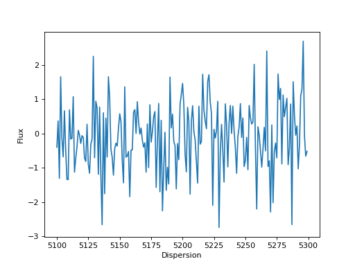
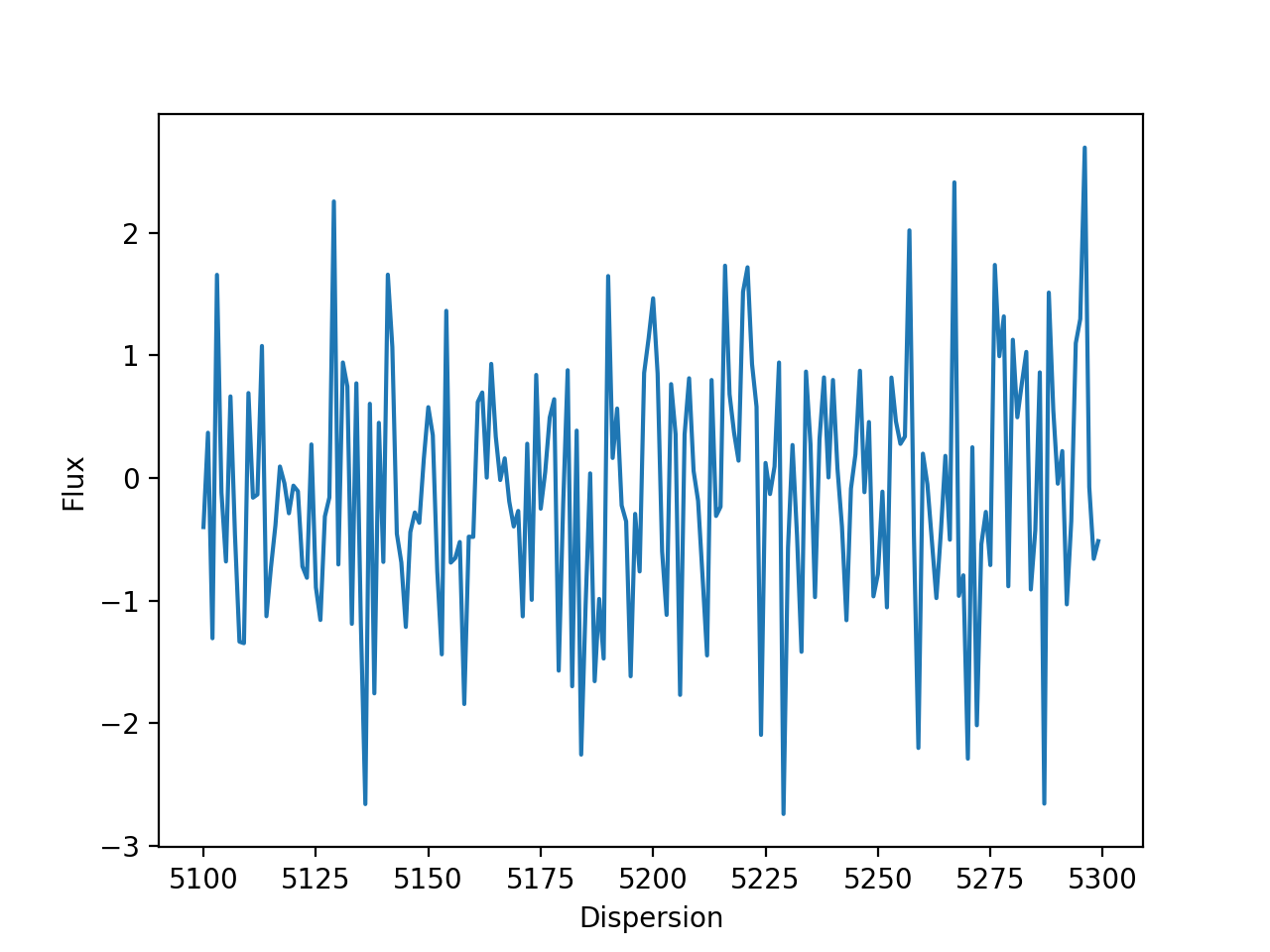
The simplest way to create a Spectrum1D is to
create it explicitly from arrays or Quantity objects:
>>> import numpy as np
>>> import astropy.units as u
>>> import matplotlib.pyplot as plt
>>> from specutils import Spectrum1D
>>> flux = np.random.randn(200)*u.Jy
>>> wavelength = np.arange(5100, 5300)*u.AA
>>> spec1d = Spectrum1D(spectral_axis=wavelength, flux=flux)
>>> ax = plt.subplots()[1]
>>> ax.plot(spec1d.spectral_axis, spec1d.flux)
>>> ax.set_xlabel("Dispersion")
>>> ax.set_ylabel("Flux")
(Source code, png, hires.png, pdf)

Note
The spectral_axis can also be provided as a SpectralAxis object,
and in fact will internally convert the spectral_axis to SpectralAxis if it
is provided as an array or Quantity.
Note
The spectral_axis can be either ascending or descending, but must be monotonic
in either case.
Reading from a File
specutils takes advantage of the Astropy IO machinery and allows loading and
writing to files. The example below shows loading a FITS file. While specutils
has some basic data loaders, for more complicated or custom files, users are
encouraged to create their own loader.
>>> from specutils import Spectrum1D
>>> spec1d = Spectrum1D.read("/path/to/file.fits")
Most of the built-in specutils default loaders can also read an existing
astropy.io.fits.HDUList object or an open file object (as resulting
from e.g. streaming a file from the internet). Note that in these cases, a
format string corresponding to an existing loader must be supplied because
these objects lack enough contextual information to automatically identify
a loader.
>>> from specutils import Spectrum1D
>>> import urllib
>>> specs = urllib.request.urlopen('https://data.sdss.org/sas/dr14/sdss/spectro/redux/26/spectra/0751/spec-0751-52251-0160.fits')
>>> Spectrum1D.read(specs, format="SDSS-III/IV spec")
<Spectrum1D(flux=[30.59662628173828 ... 51.70271682739258] 1e-17 erg / (Angstrom s cm2) (shape=(3841,), mean=51.88042 1e-17 erg / (Angstrom s cm2)); spectral_axis=<SpectralAxis [3799.2686 3800.1426 3801.0188 ... 9193.905  9196.0205 9198.141 ] Angstrom> (length=3841); uncertainty=InverseVariance)>
Note that the same spectrum could be more conveniently downloaded via astroquery, if the user has that package installed:
>>> from astroquery.sdss import SDSS
>>> specs = SDSS.get_spectra(plate=751, mjd=52251, fiberID=160, data_release=14)
>>> Spectrum1D.read(specs[0], format="SDSS-III/IV spec")
<Spectrum1D(flux=[30.59662628173828 ... 51.70271682739258] 1e-17 erg / (Angstrom s cm2) (shape=(3841,), mean=51.88042 1e-17 erg / (Angstrom s cm2)); spectral_axis=<SpectralAxis [3799.2686 3800.1426 3801.0188 ... 9193.905  9196.0205 9198.141 ] Angstrom> (length=3841); uncertainty=InverseVariance)>
List of Loaders
The Spectrum1D class has built-in support for various input and output formats.
A full list of the supported formats is shown in the table below. Note that the JWST readers
require the stdatamodels package to be installed, which is an optional dependency for
specutils.
Format |
Read |
Write |
Auto-identify |
|---|---|---|---|
6dFGS-split |
Yes |
No |
Yes |
6dFGS-tabular |
Yes |
No |
Yes |
APOGEE apStar |
Yes |
No |
Yes |
APOGEE apVisit |
Yes |
No |
Yes |
APOGEE aspcapStar |
Yes |
No |
Yes |
ASCII |
Yes |
No |
Yes |
ECSV |
Yes |
No |
Yes |
HST/COS |
Yes |
No |
Yes |
HST/STIS |
Yes |
No |
Yes |
IPAC |
Yes |
No |
Yes |
JWST c1d |
Yes |
No |
Yes |
JWST s2d |
Yes |
No |
Yes |
JWST s3d |
Yes |
No |
Yes |
JWST x1d |
Yes |
No |
Yes |
MUSCLES SED |
Yes |
No |
Yes |
MaNGA cube |
Yes |
No |
Yes |
MaNGA rss |
Yes |
No |
Yes |
SDSS spPlate |
Yes |
No |
Yes |
SDSS-I/II spSpec |
Yes |
No |
Yes |
SDSS-III/IV spec |
Yes |
No |
Yes |
SDSS-V apStar |
Yes |
No |
Yes |
SDSS-V apVisit |
Yes |
No |
Yes |
SDSS-V mwm |
Yes |
No |
Yes |
SDSS-V spec |
Yes |
No |
Yes |
Subaru-pfsObject |
Yes |
No |
Yes |
iraf |
Yes |
No |
Yes |
tabular-fits |
Yes |
Yes |
Yes |
wcs1d-fits |
Yes |
Yes |
Yes |
Writing to a File
Similarly, a Spectrum1D object can be saved to any of the supported formats using the
specutils.Spectrum1D.write() method.
>>> spec1d.write("/path/to/output.fits")
Including Uncertainties
The Spectrum1D class supports uncertainties, and
arithmetic operations performed with Spectrum1D
objects will propagate uncertainties.
Uncertainties are a special subclass of NDData, and their
propagation rules are implemented at the class level. Therefore, users must
specify the uncertainty type at creation time.
>>> from specutils import Spectrum1D
>>> from astropy.nddata import StdDevUncertainty

>>> spec = Spectrum1D(spectral_axis=np.arange(5000, 5010)*u.AA, flux=np.random.sample(10)*u.Jy, uncertainty=StdDevUncertainty(np.random.sample(10) * 0.1))
Warning
Not defining an uncertainty class will result in an
UnknownUncertainty object which will not
propagate uncertainties in arithmetic operations.
Including Masks
Masks are also available for Spectrum1D, following the
same mechanisms as NDData. That is, the mask should
have the property that it is False/0 wherever the data is good, and
True/anything else where it should be masked. This allows “data quality”
arrays to function as masks by default.
Note that this is distinct from “missing data” implementations, which generally
use NaN as a masking technique. This method has the problem that NaN
values are frequently “infectious”, in that arithmetic operations sometimes
propagate to yield results as just NaN where the intent is instead to skip
that particular pixel. It also makes it impossible to store data that in the
spectrum that may have meaning but should sometimes be masked. The separate
mask attribute in Spectrum1D addresses that in that the
spectrum may still have a value underneath the mask, but it is not used in most
calculations. To allow for compatibility with NaN-masking representations,
however, specutils will recognize flux values input as NaN and set the
mask to True for those values unless explicitly overridden.
Including Redshift or Radial Velocity
The Spectrum1D class supports setting a redshift or radial
velocity upon initialization of the object, as well as updating these values.
The default value for redshift and radial velocity is zero - to create a
Spectrum1D with a non-zero value, simply set the appropriate
attribute on object creation:
>>> spec1 = Spectrum1D(spectral_axis=np.arange(5000, 5010)*u.AA, flux=np.random.sample(10)*u.Jy, redshift = 0.15)
>>> spec2 = Spectrum1D(spectral_axis=np.arange(5000, 5010)*u.AA, flux=np.random.sample(10)*u.Jy, radial_velocity = 1000*u.Unit("km/s"))
By default, updating either the redshift or radial_velocity attributes
of an existing Spectrum1D directly uses the
specutils.Spectrum1D.shift_spectrum_to() method, which also updates the
values of the spectral_axis to match the new frame. To leave the
spectral_axis values unchanged while updating the redshift or
radial_velocity value, use the specutils.Spectrum1D.set_redshift_to()
or specutils.Spectrum1D.set_radial_velocity_to() method as appropriate.
An example of the different treatments of the spectral_axis is shown below.
>>> spec1.shift_spectrum_to(redshift=0.5)  # Equivalent: spec1.redshift = 0.5
>>> spec1.spectral_axis
<SpectralAxis
   (observer to target:
      radial_velocity=115304.79153846155 km / s
      redshift=0.5000000000000002)
  [6521.73913043, 6523.04347826, 6524.34782609, 6525.65217391,
   6526.95652174, 6528.26086957, 6529.56521739, 6530.86956522,
   6532.17391304, 6533.47826087] Angstrom>
>>> spec2.set_radial_velocity_to(5000 * u.Unit("km/s"))
>>> spec2.spectral_axis
<SpectralAxis
   (observer to target:
      radial_velocity=5000.0 km / s
      redshift=0.016819635148755285)
  [5000., 5001., 5002., 5003., 5004., 5005., 5006., 5007., 5008., 5009.] Angstrom>
Defining WCS
Specutils always maintains a WCS object whether it is passed explicitly by the
user, or is created dynamically by specutils itself. In the latter case, the
user need not be aware that the WCS object is being used, and can interact
with the Spectrum1D object as if it were only a simple
data container.
Currently, specutils understands two WCS formats: FITS WCS and GWCS. When a user does not explicitly supply a WCS object, specutils will fallback on an internal GWCS object it will create.
Note
To create a custom adapter for a different WCS class (i.e. aside from FITSWCS or GWCS), please see the documentation on WCS Adapter classes.
Providing a FITS-style WCS
>>> from specutils.spectra import Spectrum1D
>>> import astropy.wcs as fitswcs
>>> import astropy.units as u
>>> import numpy as np
>>> my_wcs = fitswcs.WCS(header={
...     'CDELT1': 1, 'CRVAL1': 6562.8, 'CUNIT1': 'Angstrom', 'CTYPE1': 'WAVE',
...     'RESTFRQ': 1400000000, 'CRPIX1': 25})
>>> spec = Spectrum1D(flux=[5,6,7] * u.Jy, wcs=my_wcs)
>>> spec.spectral_axis
<SpectralAxis
   (observer to target:
      radial_velocity=0.0 km / s
      redshift=0.0
    doppler_rest=1400000000.0 Hz
    doppler_convention=None)
  [6.5388e-07, 6.5398e-07, 6.5408e-07] m>
>>> spec.wcs.pixel_to_world(np.arange(3))
<SpectralCoord [6.5388e-07, 6.5398e-07, 6.5408e-07] m>
Multi-dimensional Data Sets
Spectrum1D also supports the multidimensional case where you
have, say, an (n_spectra, n_pix)
shaped data set where each n_spectra element provides a different flux
data array and so flux and uncertainty may be multidimensional as
long as the last dimension matches the shape of spectral_axis This is meant
to allow fast operations on collections of spectra that share the same
spectral_axis. While it may seem to conflict with the “1D” in the class
name, this name scheme is meant to communicate the presence of a single
common spectral axis.
Note
The case where each flux data array is related to a different spectral
axis is encapsulated in the SpectrumCollection
object described in the related docs.
>>> from specutils import Spectrum1D

>>> spec = Spectrum1D(spectral_axis=np.arange(5000, 5010)*u.AA,
...                   flux=np.random.default_rng(12345).random((5, 10))*u.Jy)
>>> spec_slice = spec[0]
>>> spec_slice.spectral_axis
<SpectralAxis [5000., 5001., 5002., 5003., 5004., 5005., 5006., 5007., 5008., 5009.] Angstrom>
>>> spec_slice.flux
<Quantity [0.22733602, 0.31675834, 0.79736546, 0.67625467, 0.39110955,
           0.33281393, 0.59830875, 0.18673419, 0.67275604, 0.94180287] Jy>
While the above example only shows two dimensions, this concept generalizes to
any number of dimensions for Spectrum1D, as long as the spectral
axis is always the last.
Slicing
As seen above, Spectrum1D supports slicing in the same way as any
other array-like object. Additionally, a Spectrum1D can be sliced
along the spectral axis using world coordinates.
>>> from specutils import Spectrum1D

>>> spec = Spectrum1D(spectral_axis=np.arange(5000, 5010)*u.AA,
...                   flux=np.random.default_rng(12345).random((5, 10))*u.Jy)
>>> spec_slice = spec[5002*u.AA:5006*u.AA]
>>> spec_slice.spectral_axis
<SpectralAxis [5002., 5003., 5004., 5005.] Angstrom>
It is also possible to slice on other axes using simple array indices at the same time as slicing the spectral axis based on spectral values.
>>> from specutils import Spectrum1D

>>> spec = Spectrum1D(spectral_axis=np.arange(5000, 5010)*u.AA,
...                   flux=np.random.default_rng(12345).random((5, 10))*u.Jy)
>>> spec_slice = spec[2:4, 5002*u.AA:5006*u.AA]
>>> spec_slice.shape
(2, 4)
If the specutils.Spectrum1D was created with a WCS that included spatial
information, for example in case of a spectral cube with two spatial dimensions,
the specutils.Spectrum1D.crop method can be used to subset the data based on
the world coordinates. The inputs required are two sets up astropy.coordinates
objects defining the upper and lower corner of the region desired. Note that if
one of the coordinates is decreasing along an axis, the higher world coordinate
value will apply to the lower bound input.
>>> from astropy.coordinates import SpectralCoord, SkyCoord
>>> from astropy import units as u
>>> from astropy.wcs import WCS

>>> w = WCS({'WCSAXES': 3, 'CRPIX1': 38.0, 'CRPIX2': 38.0, 'CRPIX3': 1.0,
...          'CRVAL1': 205.4384, 'CRVAL2': 27.004754, 'CRVAL3': 4.890499866509344,
...          'CTYPE1': 'RA---TAN', 'CTYPE2': 'DEC--TAN', 'CTYPE3': 'WAVE',
...          'CUNIT1': 'deg', 'CUNIT2': 'deg', 'CUNIT3': 'um',
...          'CDELT1': 3.61111097865634E-05, 'CDELT2': 3.61111097865634E-05, 'CDELT3': 0.001000000047497451,
...          'PC1_1 ': -1.0, 'PC1_2 ': 0.0, 'PC1_3 ': 0,
...          'PC2_1 ': 0.0, 'PC2_2 ': 1.0, 'PC2_3 ': 0,
...          'PC3_1 ': 0, 'PC3_2 ': 0, 'PC3_3 ': 1,
...          'DISPAXIS': 2, 'VELOSYS': -2538.02,
...          'SPECSYS': 'BARYCENT', 'RADESYS': 'ICRS', 'EQUINOX': 2000.0,
...          'LONPOLE': 180.0, 'LATPOLE': 27.004754})
>>> spec = Spectrum1D(flux=np.random.default_rng(12345).random((20, 5, 10)) * u.Jy, wcs=w)
>>> lower = [SpectralCoord(4.9, unit=u.um), SkyCoord(ra=205, dec=26, unit=u.deg)]
>>> upper = [SpectralCoord(4.9, unit=u.um), SkyCoord(ra=205.5, dec=27.5, unit=u.deg)]
>>> spec.crop(lower, upper)
<Spectrum1D(flux=[[[0.708612359963129 ... 0.6345714580773677]]] Jy (shape=(10, 5, 1), mean=0.49653 Jy); spectral_axis=<SpectralAxis
    (observer to target:
       radial_velocity=0.0 km / s
       redshift=0.0)
  [4.90049987e-06] m> (length=1))>
Collapsing
Spectrum1D has built-in convenience methods for collapsing the
flux array of the spectrum via various statistics. The available statistics are
mean, median, sum, max, and min, and may be called either on a specific axis
(or axes) or over the entire flux array. The collapse methods currently respect
the mask attribute of the Spectrum1D, but do not propagate
any uncertainty attached to the spectrum.
>>> spec = Spectrum1D(spectral_axis=np.arange(5000, 5010)*u.AA,
...                   flux=np.random.default_rng(12345).random((5, 10))*u.Jy)
>>> spec.mean()
<Quantity 0.49802844 Jy>
The ‘axis’ argument of the collapse methods may either be an integer axis, or a string specifying either ‘spectral’, which will collapse along only the spectral axis, or ‘spatial’, which will collapse along all non-spectral axes.
>>> spec.mean(axis='spatial')
<Spectrum1D(flux=<Quantity [0.37273938, 0.53843905, 0.61351648, 0.57311623, 0.44339915,
           0.66084728, 0.45881921, 0.38715911, 0.39967185, 0.53257671] Jy> (shape=(10,), mean=0.49803 Jy); spectral_axis=<SpectralAxis
   (observer to target:
      radial_velocity=0.0 km / s
      redshift=0.0)
  [5000. 5001. 5002. ... 5007. 5008. 5009.] Angstrom> (length=10))>
Note that in this case, the result of the collapse operation is a
Spectrum1D rather than an astropy.units.Quantity, because the
collapse operation left the spectral axis intact.
It is also possible to supply your own function for the collapse operation by
calling collapse() and providing a callable function
to the method argument.
>>> spec.collapse(method=np.nanmean, axis=1)
<Quantity [0.51412398, 0.52665713, 0.31419772, 0.71556421, 0.41959918] Jy>
Reference/API
Classes
|
Configuration parameters for specutils. |
|
Coordinate object representing spectral values corresponding to a specific spectrum. |
|
Spectrum container for 1D spectral data. |
|
A list that is used to hold a list of |