Working with Spectral Cubes¶

Spectral cubes can be read directly with Spectrum1D. A specific example of this is demonstrated here. In addition to the functions demonstrated below, as a subclass of NDCube, Spectrum1D also inherits useful methods for e.g. cropping based on combinations of world and spectral coordinates. Most of the functionality inherited from NDCube requires initializing the Spectrum1D object with a WCS describing the coordinates for all axes of the data.

Note that the workflow described here is for spectral cubes that are rectified such that one of the axes is entirely spectral and all the spaxels have the same spectral_axis values (i.e., case 2 in Overview of How Specutils Represents Spectra). For less-rectified cubes, pre-processing steps (not addressed by specutils at the time of this writing) will be necessary to rectify the cubes into that form. Note, though, that such cubes can be stored in specutils data structures (cases 3 and 4 in Overview of How Specutils Represents Spectra), which support some of these behaviors, even though the fulkl set of tools do not yet apply.

Loading a cube¶

We’ll use a MaNGA cube for our example, and load the data from the repository directly into a new Spectrum1D object:

>>> from astropy.utils.data import download_file
>>> from specutils.spectra import Spectrum1D
>>> filename = "https://stsci.box.com/shared/static/28a88k1qfipo4yxc4p4d40v4axtlal8y.fits"
>>> file = download_file(filename, cache=True) 
>>> sc = Spectrum1D.read(file, format='MaNGA cube') 

The cube has 74x74 spaxels with 4563 spectral axis points in each one:

>>> sc.shape 
(74, 74, 4563)

Print the contents of 3 spectral axis points in a 3x3 spaxel array:

>>> sc[30:33,30:33,2000:2003] 
<Spectrum1D(flux=[[[0.4892023205757141 ... 0.5994223356246948]]] 1e-17 erg / (Angstrom s spaxel cm2) (shape=(3, 3, 3), mean=0.54165 1e-17 erg / (Angstrom s spaxel cm2)); spectral_axis=<SpectralAxis
   (observer to target:
      radial_velocity=0.0 km / s
      redshift=0.0)
  [5.73984286e-07 5.74116466e-07 5.74248676e-07] m> (length=3); uncertainty=InverseVariance)>

Spectral slab extraction¶

The spectral_slab function can be used to extract spectral regions from the cube.

>>> import astropy.units as u
>>> from specutils.manipulation import spectral_slab
>>> ss = spectral_slab(sc, 5000.*u.AA, 5003.*u.AA) 
>>> ss.shape  
(74, 74, 3)
>>> ss[30:33,30:33,::] 
<Spectrum1D(flux=[[[0.6103081107139587 ... 0.936118483543396]]] 1e-17 erg / (Angstrom s spaxel cm2) (shape=(3, 3, 3), mean=0.83004 1e-17 erg / (Angstrom s spaxel cm2)); spectral_axis=<SpectralAxis
   (observer to target:
      radial_velocity=0.0 km / s
      redshift=0.0)
  [5.00034537e-07 5.00149688e-07 5.00264865e-07] m> (length=3); uncertainty=InverseVariance)>

Spectral Bounding Region¶

The extract_bounding_spectral_region function can be used to extract the bounding region that encompases a set of disjoint SpectralRegion instances, or a composite instance of SpectralRegion that contains disjoint sub-regions.

>>> from specutils import SpectralRegion
>>> from specutils.manipulation import extract_bounding_spectral_region
>>> composite_region = SpectralRegion([(5000*u.AA, 5002*u.AA), (5006*u.AA, 5008.*u.AA)])
>>> sub_spectrum = extract_bounding_spectral_region(sc, composite_region) 
>>> sub_spectrum.spectral_axis  
<SpectralAxis
   (observer to target:
      radial_velocity=0.0 km / s
      redshift=0.0)
  [5.00034537e-07, 5.00149688e-07, 5.00264865e-07, 5.00380068e-07,
   5.00495298e-07, 5.00610555e-07, 5.00725838e-07] m>

Moments¶

The moment function can be used to compute moments of any order along one of the cube’s axes. By default, axis=-1, which computes moments along the spectral axis (remember that the spectral axis is always last in a Spectrum1D).

>>> from specutils.analysis import moment
>>> m = moment(sc, order=1) 
>>> m.shape  
(74, 74)
>>> m[30:33,30:33]  
<Quantity [[6.45261317e-07, 6.46265069e-07, 6.48128166e-07],
           [6.46467930e-07, 6.47941283e-07, 6.51460998e-07],
           [6.48672775e-07, 6.52631872e-07, 6.56733087e-07]] m>

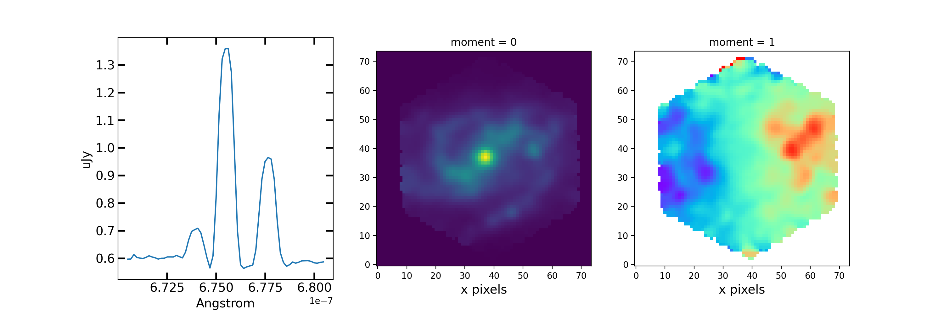
Use Case¶

Example of computing moment maps for specific wavelength ranges in a cube, using spectral_slab and moment.

import numpy as np
import matplotlib.pyplot as plt
import astropy.units as u
from astropy.utils.data import download_file
from specutils import Spectrum1D, SpectralRegion
from specutils.analysis import moment
from specutils.manipulation import spectral_slab

filename = "https://stsci.box.com/shared/static/28a88k1qfipo4yxc4p4d40v4axtlal8y.fits"
fn = download_file(filename, cache=True)
spec1d = Spectrum1D.read(fn)

# Extract H-alpha sub-cube for moment maps using spectral_slab
subspec = spectral_slab(spec1d, 6745.*u.AA, 6765*u.AA)
ha_wave = subspec.spectral_axis

# Extract wider sub-cube covering H-alpha and [N II] using spectral_slab
subspec_wide = spectral_slab(spec1d, 6705.*u.AA, 6805*u.AA)
ha_wave_wide= subspec_wide.spectral_axis

# Convert flux density to microJy and correct negative flux offset for
# this particular dataset
ha_flux = (np.sum(subspec.flux.value, axis=(0,1)) + 0.0093) * 1.0E-6*u.Jy
ha_flux_wide = (np.sum(subspec_wide.flux.value, axis=(0,1)) + 0.0093) * 1.0E-6*u.Jy

# Compute moment maps for H-alpha line
moment0_halpha = moment(subspec, order=0)
moment1_halpha = moment(subspec, order=1)

# Convert moment1 from AA to velocity
# H-alpha is redshifted to 6755 AA for this galaxy
print(moment1_halpha[40,40])
vel_map = 3.0E5 * (moment1_halpha.value - 6.755E-7) / 6.755E-7

# Plot results in 3 panels (subspec_wide,  H-alpha line flux, H-alpha velocity map)
f,(ax1,ax2,ax3) = plt.subplots(1, 3, figsize=(15, 5))
ax1.plot(ha_wave_wide, (ha_flux_wide)*1000.)
ax1.set_xlabel('Angstrom', fontsize=14)
ax1.set_ylabel('uJy', fontsize=14)
ax1.tick_params(axis="both", which='major', labelsize=14, length=8, width=2, direction='in', top=True, right=True)
ax2.imshow(moment0_halpha.value, origin='lower')
ax2.set_title('moment = 0')
ax2.set_xlabel('x pixels', fontsize=14)
ax3.imshow(vel_map, vmin=-100., vmax=100., cmap='rainbow', origin='lower')
ax3.set_title('moment = 1')
ax3.set_xlabel('x pixels', fontsize=14)

(Source code, png, hires.png, pdf)

Navigation